Graph States

Authors: Ilan Tzitrin and Luis Mantilla

A graph state is a special kind of entangled state. Certain types of graph states, called cluster states, are important resources for universal fault-tolerant quantum computation. In this tutorial we will tell you a bit about graph states, and show you how to define and visualize them using FlamingPy.

Definitions

There are a few ways of writing down a qubit graph state. We’ll split these up into graphical, operational, and through the stabilizer. The graphical definition is easiest to understand: you draw some (undirected) mathematical graph, i.e. a collection of nodes and edges, like so:

In the above graph (call it \(B\)), the nodes represent qubit states, and the edges indicate entanglement. This can be made more concrete using the operational definition: associate the nodes with \(\vert + \rangle\) states (i.e. superpositions of computational basis states: \(\frac{1}{\sqrt{2}} \left(\vert 0 \rangle + \vert 1 \rangle\right)\)), and associate the edges with \(CZ\) gates: \(\vert 0 \rangle \langle 0 \vert \otimes I + \vert 1 \rangle \langle 1 \vert \otimes Z\). This means the graph state \(\vert B \rangle\) corresponding to the graph above is:

\[\vert B \rangle = CZ (\vert + \rangle_1 \vert + \rangle_2) = \frac{1}{\sqrt{2}} \left( \vert 0 \rangle_1 \vert + \rangle_2 + \vert 1 \rangle_1 \vert -\rangle_2 \right),\]

where \(\vert - \rangle = \frac{1}{\sqrt{2}} \left(\vert 0 \rangle - \vert 1 \rangle\right)\). We can write down a circuit diagram for this:

You may recognize \(\vert B \rangle\) as a type of Bell or EPR pair: a maximally entangled state of two qubits. To create a three-qubit entangled state (equivalent to a GHZ state), we can follow the same process:

\[\vert \text{GHZ} \rangle = CZ_{23}CZ_{12} (\vert + \rangle _1 \vert + \rangle _2 \vert + \rangle _3) = \frac{1}{\sqrt{2}}(\vert 0 \rangle _1 \vert + \rangle _2 \vert + \rangle _3 + (\vert 1 \rangle _1 \vert - \rangle _2 \vert - \rangle _3)).\]

The corresponding graph and circuit are:

This is the general way entanglement is ‘’generated’’ in a graph state: the \(CZ\) gate (edge) entangles each pair of qubits (nodes).

Stabilizer definition

It is possible to completely understand graph states using the definitions above. However, it is very convenient—especially for error correction—to talk about the stabilizer of the graph state. The idea is that we can define graph states not through individual qubit states, but through operators.

In general, given a state of \(n\) qubits, you can uniquely determine the state by \(n\) distinct operators called stabilizer elements (or, colloquially, just stabilizers). When applied to the state, these operators leave the state unchanged. The stabilizers for the above states are:

\[S_B = \{X_1 Z_2, X_2 Z_1\} \qquad \text{and} \qquad S_\text{GHZ} = \{ X_1 Z_2 Z_3, Z_1 X_2 Z_3, Z_1 Z_2 X_3 \}.\]

To see this, you can use the fact that the \(Z\) operator flips phases:

\[Z \vert 0 \rangle = \vert 0 \rangle, \quad Z\vert 1 \rangle = - \vert 1 \rangle, \quad Z\vert + \rangle = \vert - \rangle, \quad Z\vert - \rangle= \vert + \rangle,\]

while the \(X\) operator flips bits:

\[X \vert 0 \rangle = \vert 1 \rangle, \quad X\vert 1 \rangle= \vert 0 \rangle, \quad X\vert + \rangle = \vert + \rangle, \quad X\vert - \rangle = -\vert - \rangle.\]

If you apply the stabilizer elements to the above states, you’ll see they don’t change. In general, if you’re given a graph state with \(n\) qubits, you can come up with \(n\) stabilizers. Each one will apply \(X\) to a given node, and \(Z\) to all the neighbours.

Creating and visualizing graph states with FlamingPy

In FlamingPy, graph states are represented through the EGraph (enhanced graph) class. Let us import this class, along with the visualization module:

from flamingpy.codes.graphs import EGraph
import flamingpy.utils.viz as viz

An EGraph is a type of (inherits from) a Graph object from the networkx package, but it builds on networkx graphs with its own functionality. EGraphs (like NetworkX graphs) have dictionaries of nodes and edges. To properly define a graph state, the EGraph class assumes that the nodes are specified by three-tuples \((x, y, z)\) corresponding to coordinates in three dimensions.

Custom graph states

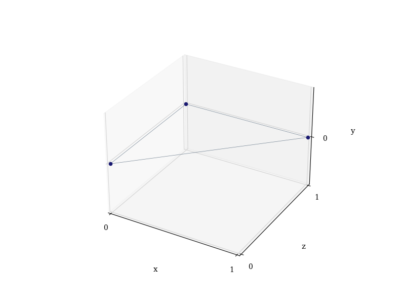
We can construct a GHZ state using FlamingPy. We can either use the built-in method complete_graph in flamingpy.utils.graph_states to obtain the EGraph of this state, or we can construct it from scratch. To do the latter, we have to place its nodes in 3D space. There are infinite choices of coordinates available to us, but let us place the points at corners of the unit cube:

GHZ_edge_1 = {(0, 0, 0), (0, 0, 1)}
GHZ_edge_2 = {(0, 0, 1), (1, 0, 1)}
GHZ_edge_3 = {(0, 0, 0), (1, 0, 1)}

We can give an EGraph its edges right away, but let us instead first initialize an empty graph:

GHZ_state = EGraph()
GHZ_state.add_edges_from([GHZ_edge_1, GHZ_edge_2, GHZ_edge_3])

Notice that there is currently nothing in the graph dictionaries except for the coordinates of the points:

print("Node attributes: ", *GHZ_state.nodes.data())
print("Edge attributes ", *GHZ_state.edges.data())

Node attributes:  ((0, 0, 0), {}) ((0, 0, 1), {}) ((1, 0, 1), {})
Edge attributes  ((0, 0, 0), (0, 0, 1), {}) ((0, 0, 0), (1, 0, 1), {}) ((0, 0, 1), (1, 0, 1), {})

Eventually, these dictionaries can be populated attributes useful for error correction and visualization. Now, we can create a plot of the state. We will first specify some drawing options, and then use the draw method of the EGraph. This is as easy as:

drawing_opts = {
    "color_nodes": "MidnightBlue",
    "color_edges": "slategray",
}
GHZ_state.draw(**drawing_opts)

(<Figure size 800x600 with 1 Axes>, <Axes3D: xlabel='x', ylabel='z', zlabel='y'>)

Built-in graph states

Now that we know how to create custom cluster states in FlamingPy, let’s use some built-in functions to generate some well-known graph states. First, we need to import the module graph_states from flamingpy.utils:

from flamingpy.utils import graph_states

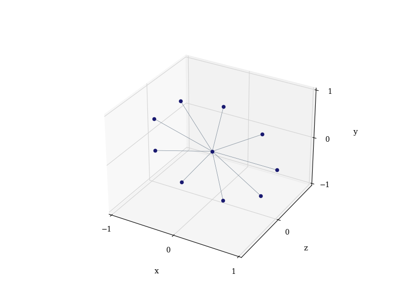
Some of the families of graph states that we have access to are star graph and complete graph states, linear cluster states (including Bell pairs as a special case), and ring or polygon states. Let us plot a star graph of 10 qubits as an example:

graph_states.star_graph(10).draw(**drawing_opts)

(<Figure size 800x600 with 1 Axes>, <Axes3D: xlabel='x', ylabel='z', zlabel='y'>)

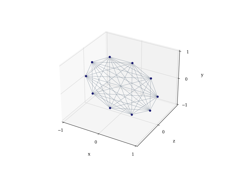
Now, let’s see how the complete graph states in 10 qubits looks like:

graph_states.complete_graph(10).draw(**drawing_opts)

(<Figure size 800x600 with 1 Axes>, <Axes3D: xlabel='x', ylabel='z', zlabel='y'>)

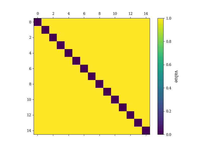
The two states above are both equivalent to GHZ states via local unitaries. We can also extract some information about the graph states, including the adjacency matrix \(A\) of the underlying graph. The indices (rows and columns) of this matrix correspond to the nodes of the graph. The entry \(A_{ij}\) is 0 if there is no edge connecting the nodes, and 1 (or another number, for weighted graphs) otherwise. We can generate the adjacency matrix and then plot its heat map:

complete_graph_state = graph_states.complete_graph(15)
complete_graph_state.draw_adj()

(<Figure size 800x600 with 2 Axes>, [<Axes: >, <Axes: label='<colorbar>', ylabel='value'>])

As expected, we have black tiles on the diagonal of the heat map, indicating no self connections (loops), and yellow tiles everywhere else, indicating maximal connectedness.

Having gone over the fundamentals of the EGraph, the representation of graph states in FlamingPy, you can better understand the structure of error correcting codes. Now, you can try to implement a resource state amenable to universal quantum computation, or check out our tutorial on error correction with the surface code: A complete round of error correction).

tutorials/_out/run_graph_states

 

Download Python script

 

Download Notebook

 

View on GitHub