Note
Go to the end to download the full example code.
A complete round of error correction
Author: Ilan Tzitrin
In this tutorial we will go over the minimal steps required to run through one round of quantum error correction: encoding, decoding, and recovery. This will allow us to demonstrate most of the functionality of FlamingPy.
The first step is to declare your choice of error-correcting code. Currently, FlamingPy gives you the option to use the surface code (also known as the planar or toric code, depending on its boundary conditions). In the measurement-based picture, the surface code is represented as a special graph state (see the graph states tutorial) called the RHG lattice. We begin by specifying some code parameters:
import matplotlib.pyplot as plt

from flamingpy.codes import SurfaceCode
from flamingpy.decoders import decoder as dec
from flamingpy.noise import IidNoise

# QEC code parameters
distance = 3
# Boundaries ("open", "toric" or "periodic")
boundaries = "open"
# Error complex ("primal" or "dual")
ec = "primal"
We will be discussing the properties of the code in more depth in another tutorial, but let us summarize them for you:
The distance of the code will correspond to size of the RHG lattice. More fundamentally, it represents the length of the smallest logical operator: a logical \(Z\) gate on the surface code, for example, will require a string of \(d\) physical \(Z\) gate on the qubits.
The
boundariesoption will determine the connectivity of the lattice at the boundary. In order to encode a single logical qubit, the boundaries must be set to ‘’open’’; this is also the choice that is more easily realizable in hardware.The error complex refers to the kind of error we would like to correct (analogous to correcting \(X\) or \(Z\) errors using the gate-based surface code). A full round of error correction involves correcting both primal and dual errors.
Having defined these parameters, we can now instantiate the code and draw it with a simple command:
# Code and code lattice (cluster state)
RHG_code = SurfaceCode(distance=distance, ec=ec, boundaries=boundaries)
RHG_code.draw()
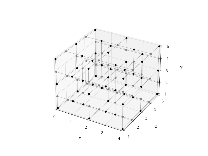
(<Figure size 800x600 with 1 Axes>, <Axes3D: xlabel='x', ylabel='z', zlabel='y'>)
By default, the primal nodes are drawn black and dual nodes as grey.
Next, we have to add some noise to our ideal qubits. For this tutorial, we opt for a simple Pauli noise model, where each qubit has some independent probability of a phase (Pauli \(Z\)) error:
At this point, we seek help from the decoder to correct our noisy lattice. The two decoders currently available in FlamingPy are minimum-weight perfect matching (‘’MWPM’’) and Union-Find (‘’UF’’). Although MWPM is slower, it is standard and well-performing; let us select it:
decoder = "MWPM"
The option "outer" here indicates that this is a qubit-level decoder
taking in bit values. One may also specify an "inner" decoder if the
qubits are, for example, GKP states, which are capable of performing an
additional round of error correction themselves. We will go over this in
more detail in another tutorial.
Finally, we can run the correct function from the decoder module, which decodes and recovers
the information. We can illustrate the full decoding procedure, for
which we first specify some drawing options:
dw = {
    "show_nodes": False,
    "color_nodes": "k",
    "show_recovery": True,
    "label_stabilizers": True,
    "label_boundary": True,
    "label_edges": False,
    "label": None,
    "legend": True,
    "show_title": True,
    "show_axes": True,
}

c = dec.correct(
    code=RHG_code,
    decoder=decoder,
    draw=True,
    drawing_opts=dw,
)
print(f"Success: {c}")
Success: True
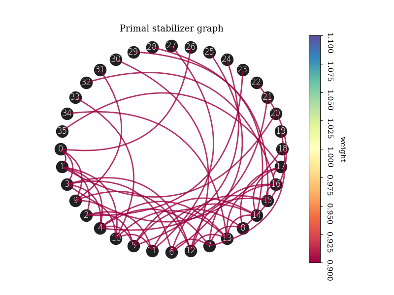
Here’s what we have drawn:
The stabilizer graph, a representation of the codes with information about the errors that have occurred.
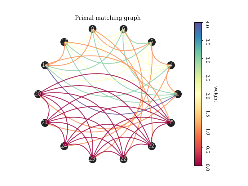
The matching graph, the processed stabilizer graph that is fed into the decoder.
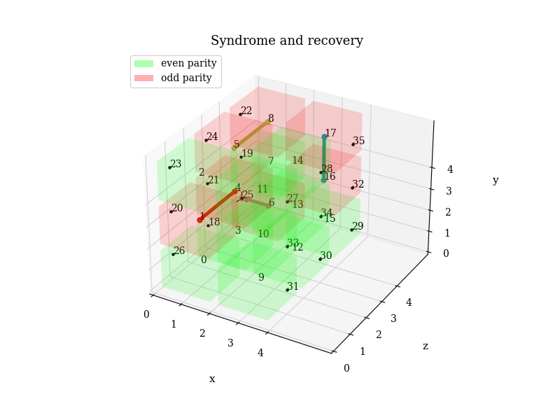
The syndrome and recovery plot, where we visualize where errors have ocurred (the red voxels) and the matching (lines connecting the voxels) that shows where the bit values must be flipped to recover the information.
You can go back and forth between these plots by comparing the indices
of the decoding graphs and those on the voxel plot. You may also display
the RHG lattice by setting "show_nodes" to True.
More information about all these steps will come in future tutorials; for now, you may visit our introduction to error correction.
Total running time of the script: (0 minutes 2.135 seconds)